Overview
The ability to dynamically render, pan, zoom, animate and perform other dynamic operations on data can provide many benefits, such as providing greater data fidelity within the same plot. HoloViz provides high-level tools (such as Holoviews, Datashader, Geoviews, etc.) to visualize even the very large datasets efficiently.
This notebook explores interactively plotting using an unstructured grid dataset in the MPAS format with Holoviews, Datashader, and Geoviews.
This notebook demonstrates:
- Use of HoloViz tools for interactive plotting
- Different interactivity schemes
- Use of the MPAS format’s connectivity information to render data on the native grid (hence avoiding costly Delaunay triangulation)
The flow of the content is as follows:
- Package imports
- MPAS preprocessing for visualization
- Utility functions
- Data loading
- Triangular mesh generation using MPAS’s cell connectivity array from the primal mesh
- Interactive Holoviz Plots
Prerequisites
| Concepts | Importance | Notes |
|---|---|---|
| Holoviews | Necessary | |
| Geoviews | Useful | Not necessary for plotting but useful for adding features |
| Matplotlib | Useful | |
| MPAS | Useful | Not necessary for interactive plotting but useful for understanding the data used |
| Xarray | Useful |
- Time to learn: 60 minutes
Imports
import math as math

import cartopy.crs as ccrs
import dask.dataframe as dd
import geocat.datafiles as gdf  # Only for reading-in datasets
import geoviews.feature as gf  # Only for displaying coastlines
import holoviews as hv
import numpy as np
import pandas as pd
from holoviews import opts
from holoviews.operation.datashader import rasterize as hds_rasterize
from numba import jit
from xarray import open_mfdataset

n_workers = 1
MPAS Preprocessing
The MPAS data requires some preprocessing to get it ready for visualization such as implementation of a few utility functions, loading the data, and creating triangular mesh out of the data to rasterize.
Utility functions
def unzipMesh(x, tris, t):
    """Splits a global mesh along longitude.

    Examine the X coordinates of each triangle in 'tris'. Return an array of 'tris' where
    only those triangles with legs whose length is less than 't' are returned.

    Parameters
    ----------
    x: numpy.ndarray
        x-coordinates of each triangle in 'tris'
    tris: numpy.ndarray
        Triangle indices for each vertex in the MPAS file, in counter-clockwise order
    t: float
        Threshold value
    """
    return tris[
        (np.abs((x[tris[:, 0]]) - (x[tris[:, 1]])) < t)
        & (np.abs((x[tris[:, 0]]) - (x[tris[:, 2]])) < t)
    ]
def triArea(x, y, tris):
"""Computes the signed area of a triangle.
Parameters
----------
x: numpy.ndarray
x-coordinates of each triangle in 'tris'
y: numpy.ndarray
y-coordinates of each triangle in 'tris'
tris: numpy.ndarray
Triangle indices for each vertex in the MPAS file
"""
return ((x[tris[:, 1]] - x[tris[:, 0]]) * (y[tris[:, 2]] - y[tris[:, 0]])) - (
(x[tris[:, 2]] - x[tris[:, 0]]) * (y[tris[:, 1]] - y[tris[:, 0]])
)def orderCCW(x, y, tris):
"""Reorder triangles as necessary so they all have counter clockwise winding order.
CCW is what Datashader and MPL require.
Parameters
----------
x: numpy.ndarray
x-coordinates of each triangle in 'tris'
y: numpy.ndarray
y-coordinates of each triangle in 'tris'
tris: numpy.ndarray
Triangle indices for each vertex in the MPAS file
"""
tris[triArea(x, y, tris) < 0.0, :] = tris[triArea(x, y, tris) < 0.0, ::-1]
return trisdef createHVTriMesh(x, y, triangle_indices, var, n_workers=1):
"""Create a Holoviews Triangle Mesh suitable for rendering with Datashader
This function returns a Holoviews TriMesh that is created from a list of coordinates, 'x'
and 'y', an array of triangle indices that addresses the coordinates in 'x' and 'y', and
a data variable 'var'. The data variable's values will annotate the triangle vertices
Parameters
----------
x: numpy.ndarray
Projected x-coordinates of each triangle in 'tris'
y: numpy.ndarray
Projected y-coordinates of each triangle in 'tris'
triangle_indices: numpy.ndarray
Triangle indices for each vertex in the MPAS file, in counter-clockwise order
var: numpy.ndarray
Data variable from which the triangle vertex values are read.
n_workers: int
Number of workers, for Dask
"""
# Declare verts array
verts = np.column_stack([x, y, var])
# Convert to pandas
verts_df = pd.DataFrame(verts, columns=["x", "y", "z"])
tris_df = pd.DataFrame(triangle_indices, columns=["v0", "v1", "v2"])
# Convert to dask
verts_ddf = dd.from_pandas(verts_df, npartitions=n_workers)
tris_ddf = dd.from_pandas(tris_df, npartitions=n_workers)
# Declare HoloViews element
tri_nodes = hv.Nodes(verts_ddf, ["x", "y", "index"], ["z"])
trimesh = hv.TriMesh((tris_ddf, tri_nodes))
return trimesh@jit(nopython=True)
def triangulatePoly(verticesOnCell, nEdgesOnCell):
"""Triangulate MPAS dual mesh:
Triangulate each polygon in a heterogenous mesh of n-gons by connecting
each internal polygon vertex to the first vertex. Uses the MPAS
auxilliary variables verticesOnCell, and nEdgesOnCell.
The function is decorated with Numba's just-in-time compiler so that it is translated into
optimized machine code for better peformance
Parameters
----------
verticesOnCell: numpy.ndarray
Connectivity array that stores the vertex indices that surround a given cell
nEdgesOnCell: numpy.ndarray
Number of edges on a given cell.
"""
# Calculate the number of triangles. nEdgesOnCell gives the number of vertices for each cell (polygon)
# The number of triangles per polygon is the number of vertices minus 2.
nTriangles = np.sum(nEdgesOnCell - 2)
triangles = np.ones((nTriangles, 3), dtype=np.int64)
nCells = verticesOnCell.shape[0]
triIndex = 0
for j in range(nCells):
for i in range(nEdgesOnCell[j] - 2):
triangles[triIndex][0] = verticesOnCell[j][0]
triangles[triIndex][1] = verticesOnCell[j][i + 1]
triangles[triIndex][2] = verticesOnCell[j][i + 2]
triIndex += 1
return trianglesLoad data and coordinates
info - Unknown Directive
info - Unknown DirectiveThe "dyamond_1" global datasets used in this example are courtesy of NCAR's Falko Judt and were produced as part of the [DYAMOND](http://dx.doi.org/10.1186/s40645-019-0304-z) initiative. They are all from the same experiment but run at several resolutions from 30km to 3.75km.
Currently, the 30-km resolution dataset is used in this example and is available at geocat-datafiles. However, the other resolutions of these data are stored on NCAR’s Glade data storage because of their size. Due to their size, the higher resolution data sets are only distributed with two variables in them:
- relhum_200hPa: Relative humidity vertically interpolated to 200 hPa
- vorticity_200hPa: Relative vorticity vertically interpolated to 200 hPa
The “relhum_200hPa” variable is computed on the MPAS ‘primal’ mesh, while “vorticity_200hPa” is computed on the MPAS ‘dual’ mesh.
# Load data
datafiles = (
    gdf.get(
        "netcdf_files/MPAS/FalkoJudt/dyamond_1/30km/diag.2016-08-20_00.00.00_subset.nc"
    ),
    gdf.get("netcdf_files/MPAS/FalkoJudt/dyamond_1/30km/x1.655362.grid_subset.nc"),
)

primalVarName = "relhum_200hPa"
dualVarName = "vorticity_200hPa"
central_longitude = 0.0

ds = open_mfdataset(datafiles, decode_times=False)
primalVar = ds[primalVarName].isel(Time=0).values
dualVar = ds[dualVarName].isel(Time=0).values

# Fetch lat and lon coordinates for the primal and dual mesh.
lonCell = ds["lonCell"].values * 180.0 / math.pi
latCell = ds["latCell"].values * 180.0 / math.pi
lonCell = ((lonCell - 180.0) % 360.0) - 180.0

lonVertex = ds["lonVertex"].values * 180.0 / math.pi
latVertex = ds["latVertex"].values * 180.0 / math.pi
lonVertex = ((lonVertex - 180.0) % 360.0) - 180.0
Generate triangular mesh using MPAS connectivity information
Primal mesh
In this example, we use the MPAS cellsOnVertex auxilliary variable, which defines mesh connectivity for the MPAS grid. Specifically, this variable tells us the cell indices contained by each cell.
So, first let’s:
- Get the triangle indices (i.e. MPAS connectivity),
- Make sure it is all in counter-clockwise order,
- “Unzip” the mesh along the longitude (for now, assuming the central longitude from the map projection is 0.0, i.e. cutting the mesh where longitude wraps around from -180.0 to 180.0)
- Project vertices from geographic to PCS coordinates
- Create Holoviews TriMesh
tris = ds.cellsOnVertex.values - 1

tris = orderCCW(lonCell, latCell, tris)

tris = unzipMesh(lonCell, tris, 90.0)

projection = ccrs.Robinson(central_longitude=central_longitude)
xPCS, yPCS, _ = projection.transform_points(ccrs.PlateCarree(), lonCell, latCell).T

trimesh = createHVTriMesh(xPCS, yPCS, tris, primalVar, n_workers=n_workers)
Dual mesh
In this example though, we use the MPAS verticesOnCell and nEdgesOnCell auxilliary variables, which defines mesh connectivity for the MPAS dual grid. A lot of details in the following code is similarv to those in the primal mesh’s case except triangulatePoly() wheere we decompose each cell into triangles since for the dual mesh, the data are located on triangle centers, which correspond to cell (polygon) vertices.
verticesOnCell = ds.verticesOnCell.values - 1
nEdgesOnCell = ds.nEdgesOnCell.values

tris_dual = triangulatePoly(verticesOnCell, nEdgesOnCell)

tris_dual = unzipMesh(lonVertex, tris_dual, 90.0)

projection = ccrs.Robinson(central_longitude=central_longitude)
xPCS_dual, yPCS_dual, _ = projection.transform_points(
    ccrs.PlateCarree(), lonVertex, latVertex
).T

trimesh_dual = createHVTriMesh(
    xPCS_dual, yPCS_dual, tris_dual, dualVar, n_workers=n_workers
)
Interactive HoloViz Plots
HoloViz tools provide essential interactivity features such as panning, zooming, hovering, clickable/selectable legends, etc. on a plot.
hv.extension("bokeh")Let’s define keyword arguments that will be commonly used for all of the plots and their opts throughout. For that, the plotting arguments are aggregator=mean to use the average of node values for shading in the rasterization and precompute=True to cache the data internally; the opts arguments are nothing more than opting in to showing the colorbar and using a colormap called “coolwarm”:
plot_kwargs = {
    "aggregator": "mean",
    "precompute": True,
}

opts_kwargs = {
    "colorbar": True,
    "cmap": "coolwarm",
}
Holoviews’ options system: opts
HoloViz packages provide high-level visualization functions that allow the customization of plot features through optional arguments. Furthermore, the HoloViews options system allows customizing a plot from title to size, legend, axes, and more. This system works by calling the .opts() method through a HoloViews plot object. We will set the opts defaults below and then customize plots throughout the notebook via .opts(). Keep an eye on them!
opts.defaults(
    opts.Image(frame_width=600, data_aspect=1),
)
Pan & zoom
Bokeh-rendered HoloViz plots come with default pan and zoom (box & wheel), tools as well as save and reset options in the very right. Just look at the following plot for those features, which uses Datashader’s rasterization method to visualize the data.
rasterized = hds_rasterize(trimesh, **plot_kwargs)
rasterized.opts(**opts_kwargs) * gf.coastline(projection=projection)
Hover
Use tools=['hover'] can be used to get the plot to display data values while hovering over the plot (there are other tools that can be selected, too, but those will not be covered in this notebook). See the below plot (let’s use the dual mesh data this time just for the sake of assortment of visualizations) and hover you cursor over it:
rasterized = hds_rasterize(trimesh_dual, **plot_kwargs)
rasterized.opts(tools=["hover"], clim=(-4e-4, 4e-4), **opts_kwargs) * gf.coastline(
    projection=projection
)
Dynamic plot
You can decide whether to return a dynamic plot that sends updates on widget and zoom/pan
events or whether all the data should be embedded by using the boolean dynamic argument.
The default value of this argument is True, so all the previously rendered plots were
already dynamic.
Now let’s look at a non-dynamic plot (i.e. dynamic=False):
rasterized = hds_rasterize(trimesh, **plot_kwargs, dynamic=False)
rasterized.opts(**opts_kwargs) * gf.coastline(projection=projection)| Non-Dynamic-Zoomed | Dynamic-Zoomed |
|---|---|
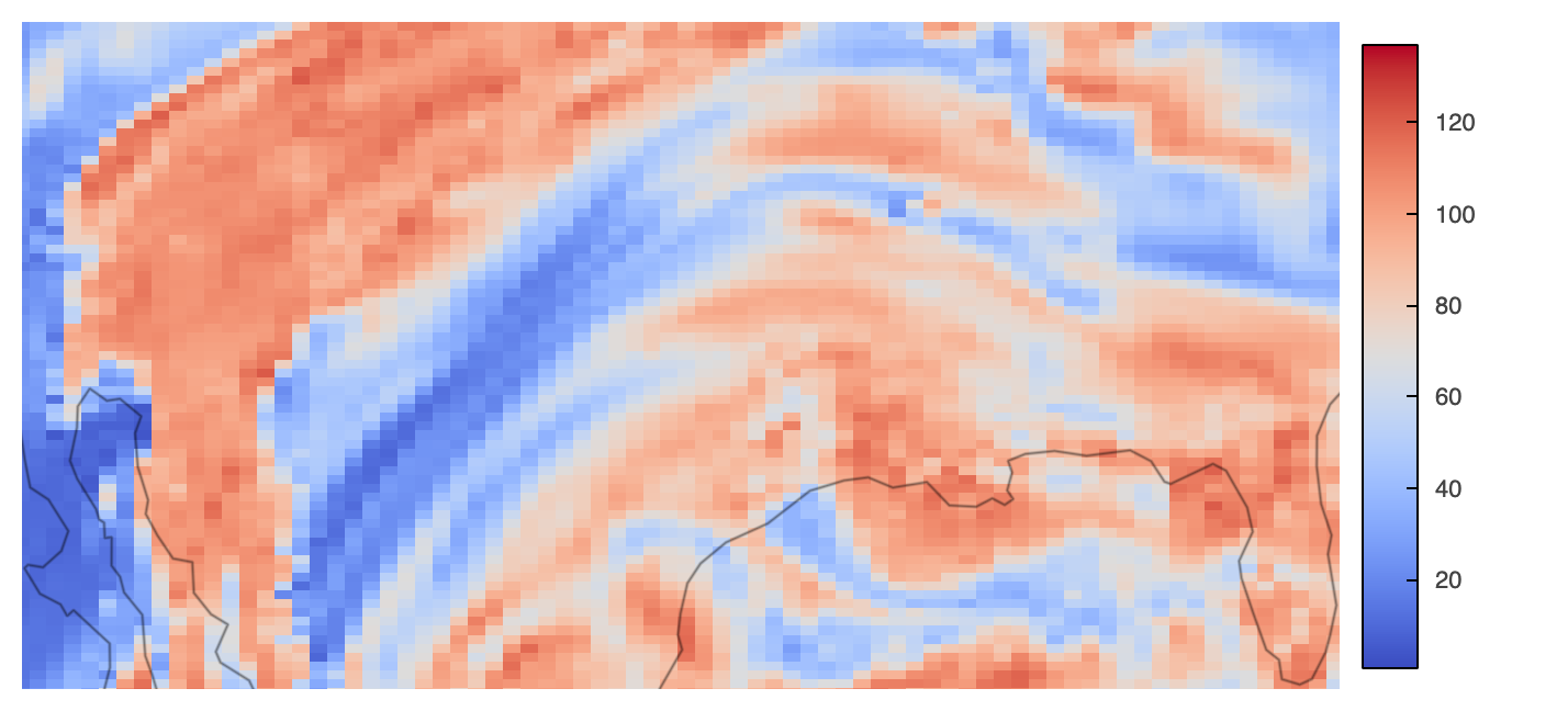 | 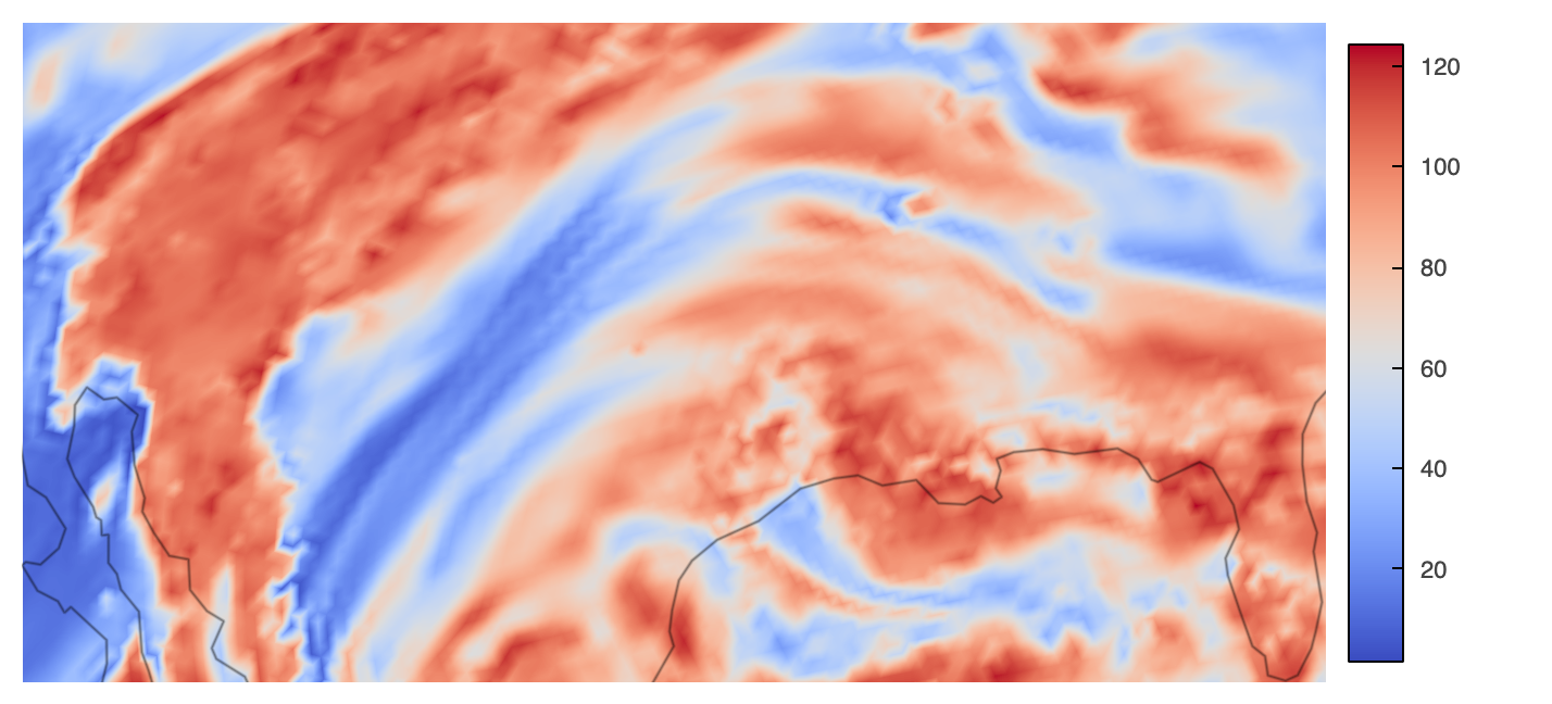 |
Further interactivity considerations
Even though we will not cover in the scope of this cookbook, you may want to have a look at the following HoloViz resources for further interactivity in your plots:
Summary
HoloViz technologies can be used in order to create interactive plots when Bokeh is used as the backend. Even though a really large dataset (e.g. km-scale) is not showcased in this notebook, HoloViz packages are reasonably performant with visualization of such data, too.
What’s next?
The end of this notebook wraps up this cookbook as well. Thanks for reading!
Resources and references
- MPAS Mesh Specification for those interested