Generate annual/yearly zarr stores from hourly ERA5 NetCDF files on NCAR’s Research Data Archive - ARCO ERA-5 Interactive Visualization Cookbook

Overview and Warning: Please Read¶

ERA5 data on NCAR is stored in hourly NetCDF files. Therefore, it is necessary to create intermediate ARCO datasets for fast processing.
In this notebook, we read hourly data from NCAR’s publicly accessible ERA5 collection using an intake catalog, compute the annual means and store the result using zarr stores.
If you don’t have write permision to save to the Research Data Archive (RDA), please save the result to your local folder.
If you need annual means for the following variables, please don’t run this notebook. The data has already been calculated and can be accessed via https from https://data.rda.ucar.edu/pythia_era5_24/annual_means/
1. Air temperature at 2 m/ VAR_2T (https://data.rda.ucar.edu/pythia_era5_24/annual_means/temp_2m_annual_1940_2023.zarr)
Otherwise, please run this script once to generate the annual means.

Prerequisites¶

Concepts	Importance	Notes
Intro to Xarray	Necessary
Intro to Intake	Necessary
Understanding of Zarr	Helpful

Time to learn: 30 minutes

Imports¶

import glob
import re
import matplotlib as plt
import numpy as np
import scipy as sp
import xarray as xr
import intake
import intake_esm
import pandas as pd

import dask
from dask.distributed import Client, performance_report
from dask_jobqueue import PBSCluster

######## File paths ################
rda_scratch       = "/gpfs/csfs1/collections/rda/scratch/harshah"
rda_data          = "/gpfs/csfs1/collections/rda/data/"
#########
rda_url           = 'https://data.rda.ucar.edu/'
era5_catalog      = rda_url + 'pythia_era5_24/pythia_intake_catalogs/era5_catalog.json'
#alternate_catalog = rda_data + 'pythia_era5_24/pythia_intake_catalogs/era5_catalog_opendap.json'
annual_means      =  rda_data + 'pythia_era5_24/annual_means/'
######## 
zarr_path         = rda_scratch + "/tas_zarr/"
##########
print(annual_means)

/gpfs/csfs1/collections/rda/data/pythia_era5_24/annual_means/

Create a Dask cluster¶

Dask Introduction¶

Dask is a solution that enables the scaling of Python libraries. It mimics popular scientific libraries such as numpy, pandas, and xarray that enables an easier path to parallel processing without having to refactor code.

There are 3 components to parallel processing with Dask: the client, the scheduler, and the workers.

The Client is best envisioned as the application that sends information to the Dask cluster. In Python applications this is handled when the client is defined with client = Client(CLUSTER_TYPE). A Dask cluster comprises of a single scheduler that manages the execution of tasks on workers. The CLUSTER_TYPE can be defined in a number of different ways.

There is LocalCluster, a cluster running on the same hardware as the application and sharing the available resources, directly in Python with dask.distributed.
In certain JupyterHubs Dask Gateway may be available and a dedicated dask cluster with its own resources can be created dynamically with dask.gateway.
On HPC systems dask_jobqueue is used to connect to the HPC Slurm and PBS job schedulers to provision resources.

The dask.distributed client python module can also be used to connect to existing clusters. A Dask Scheduler and Workers can be deployed in containers, or on Kubernetes, without using a Python function to create a dask cluster. The dask.distributed Client is configured to connect to the scheduler either by container name, or by the Kubernetes service name.

Select the Dask cluster type¶

The default will be LocalCluster as that can run on any system.

If running on a HPC computer with a PBS Scheduler, set to True. Otherwise, set to False.

USE_PBS_SCHEDULER = True

If running on Jupyter server with Dask Gateway configured, set to True. Otherwise, set to False.

USE_DASK_GATEWAY = False

Python function for a PBS cluster

# Create a PBS cluster object
def get_pbs_cluster():
    """ Create cluster through dask_jobqueue.   
    """
    from dask_jobqueue import PBSCluster
    cluster = PBSCluster(
        job_name = 'dask-pythia-24',
        cores = 1,
        memory = '4GiB',
        processes = 1,
        local_directory = rda_scratch + '/dask/spill',
        resource_spec = 'select=1:ncpus=1:mem=8GB',
        queue = 'casper',
        walltime = '1:00:00',
        #interface = 'ib0'
        interface = 'ext'
    )
    return cluster

Python function for a Gateway Cluster

def get_gateway_cluster():
    """ Create cluster through dask_gateway
    """
    from dask_gateway import Gateway

    gateway = Gateway()
    cluster = gateway.new_cluster()
    cluster.adapt(minimum=2, maximum=4)
    return cluster

Python function for a Local Cluster

def get_local_cluster():
    """ Create cluster using the Jupyter server's resources
    """
    from distributed import LocalCluster, performance_report
    cluster = LocalCluster()    

    cluster.scale(4)
    return cluster

Python logic to select the Dask Cluster type

This uses True/False boolean logic based on the variables set in the previous cells

# Obtain dask cluster in one of three ways

if USE_PBS_SCHEDULER:
    cluster = get_pbs_cluster()
elif USE_DASK_GATEWAY:
    cluster = get_gateway_cluster()
else:
    cluster = get_local_cluster()

# Connect to cluster
from distributed import Client
client = Client(cluster)

# Display cluster dashboard URL
cluster

Find data using intake catalog¶

era5_cat = intake.open_esm_datastore(era5_catalog)
era5_cat

era5_cat.df[['long_name','variable']].drop_duplicates().head()

Select variable of interest¶

######## Examples of other Variables ##############
# MTNLWRF = Outgoing Long Wave Radiation (upto a sign), Mean Top Net Long Wave Radiative Flux
# rh_cat = era5_cat.search(variable= 'R') # R =  Relative Humidity
# olr_cat = era5_cat.search(variable ='MTNLWRF')
# olr_cat
############ Access temperature data ###########
temp_cat = era5_cat.search(variable='VAR_2T',frequency = 'hourly')
temp_cat

# Define the xarray_open_kwargs with a compatible engine, for example, 'scipy'
xarray_open_kwargs = {
    'engine': 'h5netcdf',
    'chunks': {},  # Specify any chunking if needed
    'backend_kwargs': {}  # Any additional backend arguments if required
}

%%time
dset_temp = temp_cat.to_dataset_dict(xarray_open_kwargs=xarray_open_kwargs)

dset_temp.keys()

dict_keys(['an.sfc'])

temp_2m = dset_temp['an.sfc'].VAR_2T
temp_2m

temp_2m_annual = temp_2m.resample(time='1Y').mean()
temp_2m_annual

Save the notbeook¶

# temp_2m_annual.to_dataset().to_zarr(zarr_path + "e5_tas2m_monthly_1940_2023.zarr)

temp_2m_monthly = xr.open_zarr(zarr_path + "e5_tas2m_monthly_1940_2023.zarr").VAR_2T
temp_2m_monthly

temp_2m_annual = temp_2m_monthly.resample(time='1Y').mean()
temp_2m_annual = temp_2m_annual.chunk({'latitude':721,'longitude':1440})
temp_2m_annual = temp_2m_annual.drop_isel({'time':-1}) # Drop 2024 data
temp_2m_annual

Save annual mean to annual_means folder within rda_data¶

# %%time
# temp_2m_annual.to_dataset().to_zarr(annual_means + 'temp_2m_annual_1940_2023.zarr',mode='w')

CPU times: user 392 ms, sys: 26.6 ms, total: 419 ms
Wall time: 6.36 s

<xarray.backends.zarr.ZarrStore at 0x1486704723c0>

temp_2m_annual = xr.open_zarr(annual_means + 'temp_2m_annual_1940_2023.zarr').VAR_2T
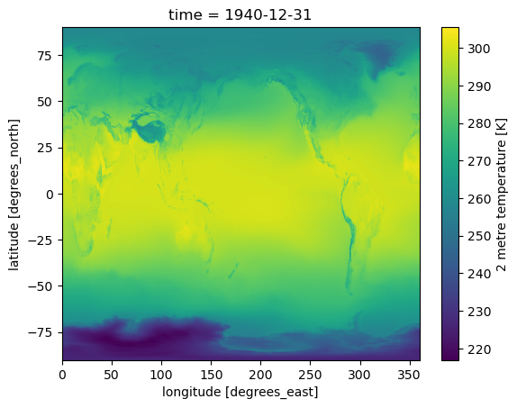
temp_2m_annual

%%time
temp_2m_annual.isel(time=0).plot()

CPU times: user 118 ms, sys: 11.5 ms, total: 130 ms
Wall time: 389 ms

Close up the cluster¶

cluster.close()

Visualization Notebooks

Creating an Interactive Dashboard using hvPlot and Panel

Preprocessing Notebooks for NCAR RDA

Access ERA5 data from NCAR’s Research Data Archive and compute anomaly