![]()


Basic Visualization using matplotlib and Cartopy
Overview
A team at Google Research & Cloud are making parts of the ECMWF Reanalysis version 5 (aka ERA-5) accessible in a Analysis Ready, Cloud Optimized (aka ARCO) format.
In this notebook, we will do the following:
- Access the ERA-5 ARCO catalog
- Select a particular dataset and variable from the catalog
- Convert the data from Gaussian to Cartesian coordinates
- Plot a map of sea-level pressure at a specific date and time using Matplotlib and Cartopy.
Imports
import fsspec
import xarray as xr
import matplotlib.pyplot as plt
import cartopy.crs as ccrs
import cartopy.feature as cfeature
import scipy.spatial
import numpy as np
import cf_xarray as cfxr
Access the ARCO ERA-5 catalog on Google Cloud
Test bucket access with fsspec
fs = fsspec.filesystem('gs')
fs.ls('gs://gcp-public-data-arco-era5/co')
['gcp-public-data-arco-era5/co/model-level-moisture.zarr',
'gcp-public-data-arco-era5/co/model-level-wind.zarr',
'gcp-public-data-arco-era5/co/single-level-forecast.zarr',
'gcp-public-data-arco-era5/co/single-level-reanalysis.zarr',
'gcp-public-data-arco-era5/co/single-level-surface.zarr']Let’s open the single-level-reanalysis Zarr file.
reanalysis = xr.open_zarr(
    'gs://gcp-public-data-arco-era5/co/single-level-reanalysis.zarr',
    chunks={'time': 48},
    consolidated=True,
)
print(f'size: {reanalysis.nbytes / (1024 ** 4)} TB')size: 28.02835009436967 TB
That’s ... a big file! But Xarray is just lazy loading the data. We can access the dataset’s metadata:
reanalysisLet’s look at the mean sea-level pressure variable.
msl = reanalysis.msl
mslThere are two dimensions to this variable ... time and values. The former is straightforward:
msl.timeThe time resolution is hourly, commencing at 0000 UTC 1 January 1979 and running through 2300 UTC 31 August 2021.
The second dimension, values, represents the actual data values. In order to usefully visualize and/or analyze it, we will need to regrid it onto a standard cartesian (in this case, latitude-longitude) grid.
Danger!
It might be tempting to run the code cellmsl.values here, but doing so will force all the data to be actively read into memory! Since this is a very large dataset, we definitely don't want to do that!Regrid to cartesian coordinates
These reanalyses are in their native, Guassian coordinates. We will define and use several functions to convert them to a lat-lon grid, using several functions described in the ARCO ERA-5 GCP example notebooks
def mirror_point_at_360(ds):
  extra_point = (
      ds.where(ds.longitude == 0, drop=True)
      .assign_coords(longitude=lambda x: x.longitude + 360)
  )
  return xr.concat([ds, extra_point], dim='values')

def build_triangulation(x, y):
  grid = np.stack([x, y], axis=1)
  return scipy.spatial.Delaunay(grid)

def interpolate(data, tri, mesh):
  indices = tri.find_simplex(mesh)
  ndim = tri.transform.shape[-1]
  T_inv = tri.transform[indices, :ndim, :]
  r = tri.transform[indices, ndim, :]
  c = np.einsum('...ij,...j', T_inv, mesh - r)
  c = np.concatenate([c, 1 - c.sum(axis=-1, keepdims=True)], axis=-1)
  result = np.einsum('...i,...i', data[:, tri.simplices[indices]], c)
  return np.where(indices == -1, np.nan, result)
Select a particular time range from the dataset
ds93 = msl.sel(time=slice('1993-03-13T18:00:00','1993-03-13T19:00:00')).compute().pipe(mirror_point_at_360)
ds93Regrid to a lat-lon grid.
tri = build_triangulation(ds93.longitude, ds93.latitude)

longitude = np.linspace(0, 360, num=360*4+1)
latitude = np.linspace(-90, 90, num=180*4+1)

mesh = np.stack(np.meshgrid(longitude, latitude, indexing='ij'), axis=-1)

grid_mesh = interpolate(ds93.values, tri, mesh)
Construct an Xarray DataArray from the regridded array.
da = xr.DataArray(data=grid_mesh,
                dims=["time", "longitude", "latitude"],
                coords=[('time', ds93.time.data), ('longitude', longitude), ('latitude', latitude)],
                name='msl')
Add some metadata to the DataArray’s coordinate variables.
da.longitude.attrs['long_name'] = 'longitude'
da.longitude.attrs['short_name'] = 'lon'
da.longitude.attrs['units'] = 'degrees_east'
da.longitude.attrs['axis'] = 'X'
da.latitude.attrs['long_name'] = 'latitude'
da.latitude.attrs['short_name'] = 'lat'
da.latitude.attrs['units'] = 'degrees_north'
da.latitude.attrs['axis'] = 'Y'da.time.attrs['long_name'] = 'time'daSelect only the first time in the DataArray and convert to hPa.
slp = da.isel(time=0)/100.Get a quick look at the grid to ensure all looks good.
slp.plot(x='longitude', y='latitude', cmap='viridis', size=7, aspect=2, add_colorbar=True, robust=True)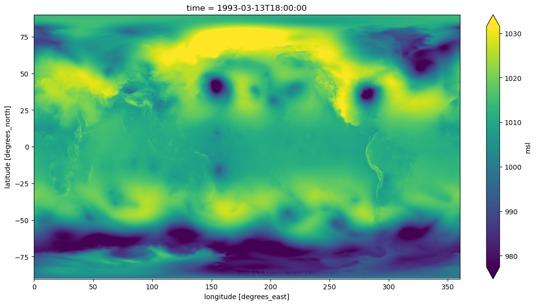
Plot the data on a map
nx,ny = np.meshgrid(longitude,latitude,indexing='ij')timeStr = '1993-03-13T18:00'
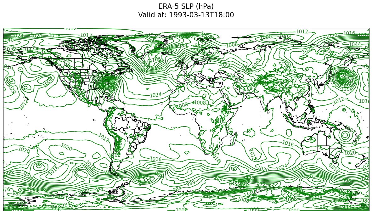
tl1 = f'ERA-5 SLP (hPa)'
tl2 = f'Valid at: {timeStr}'
title_line = (tl1 + '\n' + tl2 + '\n') # concatenate the two strings and add return characterscint = np.arange(900,1080,4)res = '50m'
fig = plt.figure(figsize=(15,10))
ax = plt.subplot(1,1,1,projection=ccrs.PlateCarree())
#ax.set_extent ([lonW+constrainLon,lonE-constrainLon,latS+constrainLat,latN-constrainLat])
ax.add_feature(cfeature.COASTLINE.with_scale(res))
ax.add_feature(cfeature.STATES.with_scale(res))
#CL = slp.cf.plot.contour(levels=cint,linewidths=1.25,colors='green')
CL = ax.contour(nx, ny, slp, transform=ccrs.PlateCarree(),levels=cint, linewidths=1.25, colors='green')
ax.clabel(CL, inline_spacing=0.2, fontsize=11, fmt='%.0f')
title = plt.title(title_line,fontsize=16)
Summary
In this notebook, we have accessed one of the ARCO ERA-5 datasets, regridded from the ECMWF native spectral to cartesian lat-lon coordinates, and created a map of sea-level pressure for a particular date and time.
What’s next?
In the next notebook, we will leverage the Holoviz ecosystem and create interactive visualizations of the ARCO ERA-5 datasets.
Resources and references
- This notebook follows the general workflow as used in the Google Research ARCO-ERA5 Surface Reanlysis Walkthrough notebook
- Stern, C., Abernathey, R., Hamman, J., Wegener, R., Lepore, C., Harkins, S., & Merose, A. (2022). Pangeo Forge: Crowdsourcing Analysis-Ready, Cloud Optimized Data Production. Frontiers in Climate, 3. 10.3389/fclim.2021.782909